Signal
Processing has undergone a revolution over the past half
century. In my youth, radios were made of discrete electronic components,
typically 5 or 6 vacuum
tubes and various other
components, wires, condensers (capacitors), half-watt or larger
resistors,
a couple of mysterious tin cans (IF transformers), and an air-variable
tuning capacitor—if you touched the latter when the radio was on, you
would remember the experience.
Now radio receivers consist
mainly of
software—of course some hardware is needed to run the software, one
or more microprocessors and memory, etc. Hardware is also
necessary where signals come in. (You cannot make an antenna
out of software—not yet, anyway.)
The
dividing line between hardware and software is somewhat variable. You
can see how this would be so by thinking about the
simplest radio receiver—a crystal set (or the proverbial tooth filling).
SDR
Hardware Study: The hardware
part of Software Defined Radio (SDR), which is the focus of
this project,
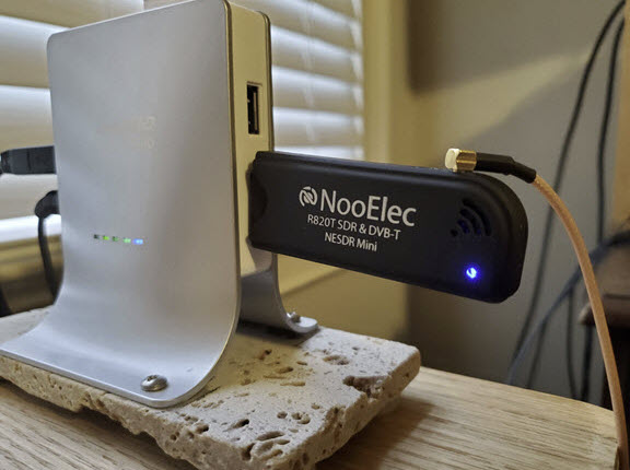
is a solved problem. Inexpensive consumer devices are commonly available.
For less than $25 one can purchase a DVB-T SDR. These devices plug into
a computer USB port the same as thumb
drives. By comparison, state-of-the-art software defined communications
receivers can cost in the thousands or even tens of
thousands of dollars. However, the point of the present
exercise is not to survey professionally engineered devices, but
rather to gain a better understanding of SDR concepts through hands-on
exploration.
I had read several instructive articles
about SDR
hardware, as well as a few book chapters.1
This article about the RTL-SDR
dongle was particularly helpful. However, an entirely
satisfactory understanding would require a high tolerance for math, or
better,
a love of the subject. I am not an engineer, so
technical articles, which often include jargon as well as
moderately advanced math, can be daunting. On the other hand, working
with a soldering iron can also contribute to understanding.
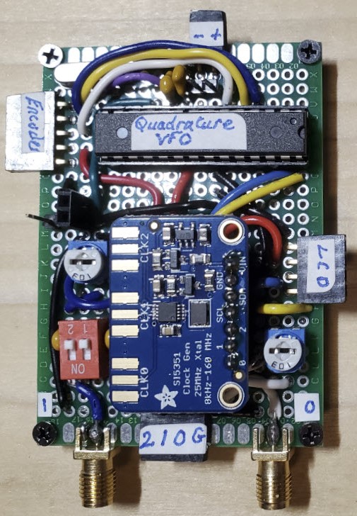 Quadrature
VFO: A previous project had made me aware of Eero Kyllonen OH2BTG’s I/Q VFO.
Somehow I returned to this page and wondered if the quadrature
VFO would be a good starting point for the present
exploration. A regular VFO has one output, while a quadrature VFO has
‘I’ and ‘Q’ outputs.2
Both outputs have precisely the same frequency, but one lags the other
by
90°. In OH2BTG’s I/Q VFO
the CLK0 and CLK1 outputs of a SI5351 Clock Generator are programmed to
satisfy this requirement.
Quadrature
VFO: A previous project had made me aware of Eero Kyllonen OH2BTG’s I/Q VFO.
Somehow I returned to this page and wondered if the quadrature
VFO would be a good starting point for the present
exploration. A regular VFO has one output, while a quadrature VFO has
‘I’ and ‘Q’ outputs.2
Both outputs have precisely the same frequency, but one lags the other
by
90°. In OH2BTG’s I/Q VFO
the CLK0 and CLK1 outputs of a SI5351 Clock Generator are programmed to
satisfy this requirement.
I
did not modify any important part of OH2BTG’s
Arduino sketch
(MPU program). A comment
in the original sketch
acknowledges Hans Summers and others for
contributing help and code. While I did not change the frequency and
phase control code, I did adapt the sketch to use an i2c-interfaced
LCD and also to
store
frequency and the frequency step in EEPROM for recall after
power cycling.
These were ‘convenience’ modifications.
The I/Q VFO sketch
documents
3.3 MHz to 58 MHz as the frequency range for which ‘I’ and ‘Q’ outputs
are orthogonal. I observed (confirmed) the phase
difference directly at the Si5351 clock outputs from just below 3.3
MHz to around 15 MHz. (I did not test higher frequencies.) However,
from previous experience with the
Si5351, I knew
that output level would vary substantially across the clock generator’s
frequency range,
being much greater at low
frequencies than toward the upper end of the range. Therefore I
installed a pair of potentiometers for the purpose of adjusting
levels and balancing outputs. I also added a pair of DIP
switches to select between DC or AC coupling.
Mixers:
At this stage of the
project I was
pleased to have constructed something that worked, and would have been
content to
hang the project up. But then the thought occurred that a responsible
person would likely carry on to the mixer stage before quitting. The
parts bin (actually a rack of
labeled drawers) contained several NE602AN double-balanced mixer IC's
left over from bygone projects. However, an on-line search for
alternatives turned
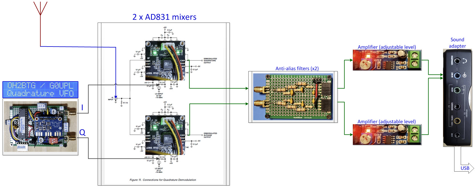
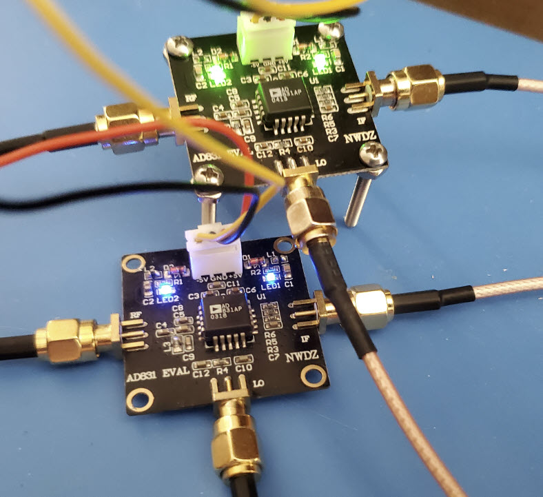
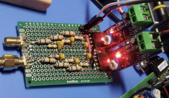
up the Analog Devices AD831. On skimming the AD831 datasheet,
I was seduced by a diagram on page 12 titled, “Connections for
Quadrature Demodulation.” (The same diagram is part of the project
illustration at the top of this page, with photos of the
evaluation boards pasted over the AD831’s).
While waiting for delivery of AD831 eval
boards I began to think how the setup could be tested. I was not yet
aware of Alberto Di Bene’s
(I2PHD) SDRadio, and imagined having to contrive something
with Gnuradio Companion.
Anticipating this option I installed the latest version of gnuradio.
This was a mistake. The
grc block
specification format had changed from .xml to .yaml. At
least a full day was lost trying to recover
source
blocks that had been available in the previous install
version. Nothing that I tried restored the missing blocks,
so I really did abandon
that plan—for now.
 Anti-alias
filters: Mixers
mix—they combine RF and local oscillator signals to produce both
the sum and difference of these waves. After mixing, the useable part
of analog output from the mixer (IF) has to be sampled (converted to
digital
form) for input to the computer application. An important factor
affecting how much IF bandwidth can be processed by the computer
application is the speed with which
analog-to-digital conversion can be accomplished. Present day
state-of-the-art A/D converters are fantastically fast, but that fact
is not particularly germane to my project, as I intended to use a sound
card for A/D conversion. Sound-card sampling rates are measured
in kilo-samples per second KSa/s, not MSa/s.
Anti-alias
filters: Mixers
mix—they combine RF and local oscillator signals to produce both
the sum and difference of these waves. After mixing, the useable part
of analog output from the mixer (IF) has to be sampled (converted to
digital
form) for input to the computer application. An important factor
affecting how much IF bandwidth can be processed by the computer
application is the speed with which
analog-to-digital conversion can be accomplished. Present day
state-of-the-art A/D converters are fantastically fast, but that fact
is not particularly germane to my project, as I intended to use a sound
card for A/D conversion. Sound-card sampling rates are measured
in kilo-samples per second KSa/s, not MSa/s.
A famous mathematical theorem asserts
that in order to reconstruct a sampled wave perfectly, the sampling
rate must be more than twice the highest frequency component in the
wave. The wave reconstruction process connects dots, similar to the way
a
child connects dots in a coloring book to make a picture. If there are
many closely spaced dots the picture will be smooth (or smoother). But
if there are too few dots the picture might look edgy or indeed it may
be impossible to figure out what the
picture was
supposed to represent. Intuitively,
the more dots there are, the
smoother the representation of the wave.
When the reconstruction process
misclassifies frequencies that are too fast for the sampling rate, the
error is called ‘aliasing’ and that is why the low-pass filters in the
project diagram are called ‘anti-alias’ filters. Many explanations of
aliasing can be found on-line. This
one is particularly readable and nicely illustrated. To be
fair, the connect-the-dots analogy of the previous paragraph
is not the full story. In the reconstructive part of signal processing
dots are
connected, not by straight line segments, but by a special function
that ensures fidelity when the sampling rate requirement is satisfied.
That this procedure works
seems magical!3
Although some computer sound cards are
capable of faster sampling rates, most sample at either 44,100 Sa/sec
or
48,000 Sa/sec. Therefore I constructed low-pass filters for just over
20,000 Hz, less than half the anticipated sampling rate. This on-line calculator was used
to pick
appropriate R and C values for -3dB per filter stage. Three stages of
low-pass
filtering attenuates the signals, so amplifiers and
gain potentiometers were
added. In retrospect it might have been possible to
use the
sound card’s stereo microphone input, skipping the amplifiers, but I
was fixated on using line-in at the time.
Back to
mixers: The mixer evaluation boards require both negative
and positive power supplies, ±5 VDC. To satisfy this requirement
I used 6 AA batteries, tapped in the middle, for −4.5 and +4.5
VDC, a
little more when the batteries were fresh, and less after a few hours!
The AD831 datasheet says 200 mV to 1 volt (P-P) for the local
oscillator inputs, so VFO outputs were set to 500 mV for
connection to the AD831’s.
To bench-test each mixer, I connected a short insulated wire (a
breadboard
jumper) to
the SMA antenna input and ran the IF output through one of the
filter-amplifiers. A small speaker was connected to the amplifier
output. A 1-volt P-P test signal (produced by a function generator) was
coupled to a ferrite loop antenna. The receive antenna was placed very
close to the loop so that a
beat tone could be heard from the speaker when function generator
and VFO
frequencies were a few hundred Hertz apart.
Filter output amplifiers were adjusted
to make the
beat tone approximately the same volume
(by ear) from both mixers. Later I
increased the
volume, but kept the outputs in balance. These preliminary
exercises revealed no surprises, although with three power supplies and
the
function generator output button, I sometimes forgot to switch-on one
of
the
components, resulting in
a momentary twinge of concern.
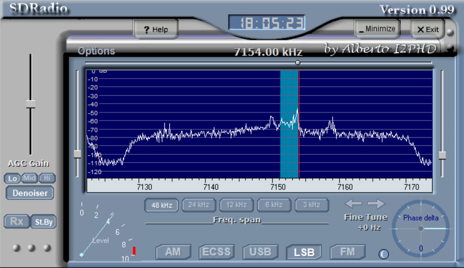
SDRadio:
This project would still be languishing at the bench-test phase if it
were not for I2PHD’s SDRadio. This fine application enables a
more-or-less realistic test of the hardware configuration. SDRadio
accepts
digitized IQ input from an ordinary sound card. Thus, only a sound card
driver
is needed, nothing special. This Windows program provides a compatible
or
generic test platform, perfect for amateur experimentation. For
interfacing with SDRadio, I
used an older Sewell external USB sound card—cannot
find the specific model on-line—any
sound card should
do. The sound card’s left
and right stereo channels correspond to the ‘I’ and ‘Q’ channels of the
sampled waveform. Also, for this demonstration, a real antenna
(dipole) was connected to the dual mixer inputs using a short SMA
splitter.
In the screen shot above, an LSB
station was tuned at 7154 KHz. Several other signals are visible in
the spectrum between about 7130 and 7170 KHz.
I should point out that SDRadio does not control the tuner (VFO).
However, SDRadio can be made to display the true frequency by setting
the center
frequency of its display to the selected VFO frequency.4
In the video
demo that accompanies this write-up, displayed frequencies are true
(i.e., synchronized with the VFO).
Demo
video: Testing
the SDR
1. The book chapters came from Communications Receivers
(Fourth Edition) by Rohde, Whitaker, and Zahnd; and Digital Signal Processing
by Steven W. Smith.
2. ‘I’ and ‘Q’ stand for ‘In-phase’
and ‘Quadrature’. (In the signal processing context, the term ‘IQ’ has
nothing to do with
Intelligence Quotient!) While the project summary on this page skirts
technical aspects
of signal processing, mathematics cannot be avoided in the quest for
genuine
understanding . For example, the mixer function can be
understood
in relation to an elementary trigonometric identity. While
anti-aliasing and
A-D sampling steps are based on the Nyquist-Shannon sampling theorem,
and processing of digitized quadrature IF output (SDRadio) involves the
complex DFT and other advanced methods.
3. The ‘magic’ interpolation
function is
sinc(x) = sin(x)/x.
4. In quadrature configuration, the
mixer output may be regarded as a complex wave with Cartesian
coordinates I (real) and Q (imaginary). —The complex DFT
includes negative
frequencies, hence the ±tuning range.
Project descriptions on this page are intended for entertainment only.
The author makes no claim as to the accuracy or completeness of the
information presented. In no event will the author be liable for any
damages, lost effort, inability to carry out a similar project, or to
reproduce a claimed result, or anything else relating to a decision to
use the information on this page.