QRP SWR Meter

 Minimalist radio transmitters: I had been
playing with a couple of exceedingly simple transmitters, the so-called
Ten-Minute Transmitter and the
Michigan Mighty Mite. Both are
single-transistor, very low power transmitters, bare minimum designs,
so-to-speak. By
connecting each unit’s RF output to a dummy load, and
listening on a nearby receiver, it is easy to confirm that they do in
fact transmit.
When powered from a 9-volt battery, the
Mighty Mite puts out about 60 milliwatts RMS (as ascertained by
measuring
RF voltage
across a resistive load).
Minimalist radio transmitters: I had been
playing with a couple of exceedingly simple transmitters, the so-called
Ten-Minute Transmitter and the
Michigan Mighty Mite. Both are
single-transistor, very low power transmitters, bare minimum designs,
so-to-speak. By
connecting each unit’s RF output to a dummy load, and
listening on a nearby receiver, it is easy to confirm that they do in
fact transmit.
When powered from a 9-volt battery, the
Mighty Mite puts out about 60 milliwatts RMS (as ascertained by
measuring
RF voltage
across a resistive load).
According to Wikipedia,
the term ‘QRP’
generally refers to
5 watts or less power in CW mode,
e.g., Morse code. Interestingly, milliwatt-range transmitters have
their own sub-designation. Transmitters that produce 1 watt or less are
sometimes referred to as ‘QRPp’.
Enthusiasts of this exeptionally low power range strive to make contact
over impressive and occasionally spectacular distances, using minimal
power. —But
I digress. Making
and testing these
small transmitters caused me to wonder whether their output would
suffice to produce meaningful readings on a power / SWR meter. That
thought
led to purchasing an inexpensive QRP
SWR Bridge from Kits And Parts (.com). This small kit
requires only an hour or two to assemble and test.

 Balancing the bridge:
The last step in the KitsAndParts.com build instructions
explains how to produce equal readings for the same power and load,
whether connected in the forward or reverse direction. Each
arm of the
bridge has a
variable resistor that can be trimmed to increase or decrease
the value displayed on a DC microammeter (for a given RF input
and
load).
After adjusting for a suitable reading in the forward direction,
connect the RF source to the output (antenna) side of the bridge and a
dummy load
to the input; then adjust the ‘reverse’ trimmer until the meter
displays the same value as it did for the forward-connected power and
load.
Balancing the bridge:
The last step in the KitsAndParts.com build instructions
explains how to produce equal readings for the same power and load,
whether connected in the forward or reverse direction. Each
arm of the
bridge has a
variable resistor that can be trimmed to increase or decrease
the value displayed on a DC microammeter (for a given RF input
and
load).
After adjusting for a suitable reading in the forward direction,
connect the RF source to the output (antenna) side of the bridge and a
dummy load
to the input; then adjust the ‘reverse’ trimmer until the meter
displays the same value as it did for the forward-connected power and
load.
Calibration: By all rights a power
meter should display units of power: watts or
milliwatts, or, if you’re the power company, megawatts! Although the
QRP
SWR  bridge
was advertised for the range 5 to 100 watts there was a
chance that it
might also function down to the fractional-watt range of the
one-transistor transmitters.
To explore this possibility I adjusted both forward and
reverse
arms of the bridge to their maximum
sensitivity
points—trimpots nearly fully clockwise—before proceeding. The next step
or goal was to interface the bridge with an Arduino Nano. The Nano
platform could be used for reading voltage and displaying power in
appropriate
units, as well as Standing Wave Ratio.
bridge
was advertised for the range 5 to 100 watts there was a
chance that it
might also function down to the fractional-watt range of the
one-transistor transmitters.
To explore this possibility I adjusted both forward and
reverse
arms of the bridge to their maximum
sensitivity
points—trimpots nearly fully clockwise—before proceeding. The next step
or goal was to interface the bridge with an Arduino Nano. The Nano
platform could be used for reading voltage and displaying power in
appropriate
units, as well as Standing Wave Ratio.
With a 5-watt transceiver1 supplying RF
input, voltage at the microammeter connection point of the
bridge was low enough to be connected
safely
to
a Nano’s analog-to-digital (A/D) input. The bridge output was around
half 3.3
volts. Thus, substituting 3.3 volts as the analog reference (Nano
A-ref pin), in place of the default 5 volts, was expected to enhance
the measurement’s digital resolution.
The test transceiver’s RF power output varies with the power
supply
voltage. Thus by setting the DC input to different values, and
recording
A/D readings for each power supply level tested, it was possible to
establish a correlation between
A/D values (bridge output) and RF
power (as calculated from peak-to-peak RF voltage across a
50-ohm
resistive load).2
Important note:
The following table and accompanying linear regression graph have been
revised to correct an error that was discovered after first posting
this
write-up. When raw A/D values were originally measured,
the analogReference(EXTERNAL) specification had been omitted
from the microcontroller sketch; hence the reference voltage was
not stable. The sketch
(see links below) has also been corrected.

The preceding table contains just three
measurement points. However, the
xy-graph of power versus raw A/D (below) shows that a straight line
through the points provides satisfactory accuracy
for
this limited measurement range.
The calculator
at https://www.socscistatistics.com/tests/regression/default.aspx
was used to compute the line’s slope and intercept.

While it might have been better to define two
lines, one for the the illustrated QRP range and another for
the
milliwatt range, at this stage of the
project I was ready to move on to the user interface. (But
see ‘QRPp addendum’ and
subsequent paragraphs below.)
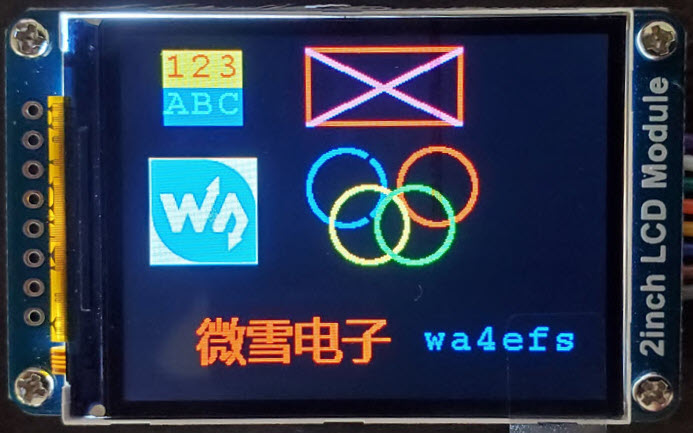
Displaying power and SWR: At first a
two-line (16×2)
text-only LCD was used to
observe raw A/D (calibration) readings, and for
displaying measured RF power and SWR (topmost illustration).
This non-graphic display interfaces via
the i2c bus. I had previously
interfaced the same type of LCD to the test transceiver itself
(Hilltopper-40) in order to
display tuned frequency and
step, etc. It might be possible, I thought, to extend the Hilltopper’s
MPU code
again, this time to include
power and SWR information, along with frequency, and so forth, using
the same
2-line
display. However,
there was a
hitch. Only one of the transceiver’s ATmega328P analog pins remained
unassigned—marked as ‘spare’ in the schematic. All other analog
channels were in use. I briefly
considered
multiplexing forward and reverse power data to the last available
analog
channel, but discarded this idea, and in its place began to
entertain a
more grandiose one!
 Virtual meter:
Why not paint a cross-needle meter face on a pixel-addressable device
and have the display emulate an analog SWR meter? This idea seemed
entirely
feasible. It was similar in concept to my OLED-based magic
eye simulation. Casting about for a suitable display, I took
a $15 chance and ordered a Waveshare 2-inch color LCD
(240×320) pixels. Two
inches seemed about right—A
QRP meter should be small, like other QRP
devices.
Virtual meter:
Why not paint a cross-needle meter face on a pixel-addressable device
and have the display emulate an analog SWR meter? This idea seemed
entirely
feasible. It was similar in concept to my OLED-based magic
eye simulation. Casting about for a suitable display, I took
a $15 chance and ordered a Waveshare 2-inch color LCD
(240×320) pixels. Two
inches seemed about right—A
QRP meter should be small, like other QRP
devices.
The Waveshare LCD module
connects via the
Serial Peripheral Interface and is furnished with a custom SPI cable.
Somehow I had
imagined
programming this display using
a rich graphics library, similar to the Adafruit GFX library that had
been used for the magic
eye sketch.
This was a misapprehension, or rather a pipe-dream. On
first exercising the Waveshare
demo
(slightly customized in the photo left) I became aware of how
slowly
the device
paints, and soon realized that it would not be feasible to simulate
cross-needles with real-time motion, at least not if relying
on the Waveshare
demonstration files for drawing functions.

 Meter bars: If the imagined
cross-needle display could not be readily implemented, surely it would
be possible to update graphic meter bars to reflect forward and
reflected
power, and SWR, in real time. Such a display would consist
of horizontal rectangles, like progress bars, that fill up to
an indicated value (photo left). Updating
would be
simple—fill more to the right when changing to a greater value, or
erase to the left (i.e., fill with the background color) for a
decreasing value. Alas, this much simpler plan was also too slow when
the value to be displayed changed more than fractionally. Reluctantly I
gave up the ‘fill’ concept and
in its place made a single vertical mark at the position to be
indicated
(photo right). A
3-pixel wide mark was sufficiently salient, and at the same time
could be painted or erased relatively quickly.
Meter bars: If the imagined
cross-needle display could not be readily implemented, surely it would
be possible to update graphic meter bars to reflect forward and
reflected
power, and SWR, in real time. Such a display would consist
of horizontal rectangles, like progress bars, that fill up to
an indicated value (photo left). Updating
would be
simple—fill more to the right when changing to a greater value, or
erase to the left (i.e., fill with the background color) for a
decreasing value. Alas, this much simpler plan was also too slow when
the value to be displayed changed more than fractionally. Reluctantly I
gave up the ‘fill’ concept and
in its place made a single vertical mark at the position to be
indicated
(photo right). A
3-pixel wide mark was sufficiently salient, and at the same time
could be painted or erased relatively quickly.
In
addition to labeled meter bars, the revised LCD screen geometry
features a
single row of text at the
bottom. This part of the display was subsequently extended to include a
numeric value for
forward power, in addition to the illustrated SWR.
Detecting key-down:
It seemed
that the display should change, maybe blank-out, during the receive
part of transceiving. To test this idea, it was necessary to implement
key-down detection, which in turn involved routing a cable
from the transceiver to convey ‘Txen’ (transmit enable) and
‘Mute’
signals to designated Nano digital inputs. Although analog SWR meters
do not disconnect during receive, modern ham radio transceivers do
support selection of
different
virtual
meters for the two parts of the transceive cycle. For example an
S-meter may be displayed on receive, and ALC or power or SWR on
transmit. However, this concept
ran up against the same problem as updating meters. The Waveshare
2-inch LCD screen can not
be repainted fast enough to switch between different transmit and
receive displays, even
if programmed to preserve the transmit-mode display for a brief
interval
after
key-up. The dual-display idea was abandoned.

Simulating the bridge: Every change to
the display required modifying microcontroller code, though usually in
a minor way. Having to repeatedly fire up and key the transceiver in
order to test such changes became a chore. To speed things up I made a
simulator
consisting of
two voltage dividers (50K trimmer potentiometers), one connected to the
forward power analog input pin (A0) of the Nano and the other to the
reflected power pin
(A1). This simple expedient, which bypasses the transceiver and bridge,
facilitated more efficient
testing
of code
changes.
Wrap-up: The project software (sketch or
program) may be
examined or downloaded
from this
page. It is important to realize that calibration
constants are peculiar to the specific implementation described in
these paragraphs.
Adapting
the
sketch for a different SWR bridge would necessarily require calibration
with the
bridge
that is to be connected. By the same token, it might be necessary
to use a different analog reference voltage (A-ref) or to condition
the bridge output level for connection with the MPU, etc. Also
note
that the LCD_Driver.h
and GUI_Paint.h library files, cited in the accompanying sketch’s
conditional compile directives, must be
downloaded separately from Waveshare along with the accessory C++ font
files. These Waveshare demonstration resources are not part of the
project sketch download. The purpose of posting the sketch
in
its current form is to share implementation ideas, not necessarily for
reproducing the project verbatim.
When very low power one-transistor
transmitters
(first paragraph above)
are tested, the 0 to 10 watt forward power meter bar only
sometimes moves, and then barely away from zero. For these
transmitters, the bottom line textual display
reports power in milliwatts. Such low values are likely inaccurate—they
are
certainly highly
variable. On the other hand
it is possible to simulate ‘QRPp’ values in a reproducible way,
using the A-ref
voltage dividers (breadboard photo above). Perhaps
also the bridge itself
could be
made more sensitive if intended chiefly for use in a milliwatt
application.
 QRPp (addendum): After correcting the omission
of the analogReference(EXTERNAL) statement in the sketch, it became
feasible to set the A-ref voltage to less than 3.3 volts, in the hope
of improving measurement sensitivity at lower power levels, and perhaps
to
test whether this concept could be applied to make reproducible
measurements of the milliwatt transmitters’ RF power output.
QRPp (addendum): After correcting the omission
of the analogReference(EXTERNAL) statement in the sketch, it became
feasible to set the A-ref voltage to less than 3.3 volts, in the hope
of improving measurement sensitivity at lower power levels, and perhaps
to
test whether this concept could be applied to make reproducible
measurements of the milliwatt transmitters’ RF power output.
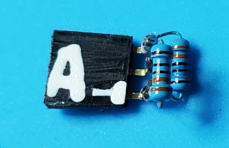
My first thought was to use a 1 volt
Zener diode, but the smallest Zener on hand was marked 3 volts.
According to https://skillbank.co.uk/arduino/measure.htm
the Arduino A-ref pin has an internal resistance of 32K ohms.
Therefore, it should be possible to use a voltage divider to derive a
stable lower voltage reference from the Nano’s 3.3 volts. With two 330
ohm resistors to halve the voltage, the current draw would be
only 5 ma. As a first step I installed a pin header on the Nano
sub-board in place of the 3.3 volts-to-A-ref jumper, so that additional
test voltages could be conveniently substituted for the originally
calibrated one. The photo shows two 1% resistors configured to supply
1.65 volts to the A-ref pin. The third pin header pin connects to
ground. Note that this female header plugs into the sub-board, not to
the Nano itself, where its ground pin would align incorrectly with DIO
13.
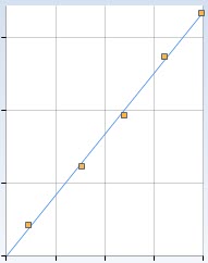 With A-ref = 1.65
volts the A/D range is roughly doubled. Five data points in the range
1.5 to 3 watts (RMS power) were used for calibrating at this
sensitivity, and the fit remained essentially linear (figure right). To
accommodate this lower power range the sketch was modified to include a
new Boolean constant QRPp, which if initialized ‘true’ would substitute
the enhanced sensitivity regression equation in place of the default one (for example, ŷ = 0.01x -
2.91 for the particular bridge adjustment and 1.65 volt A-ref tested).
This sketch revision may be examined or downloaded here.
Once again it must be stressed that slope and intercepts listed in the
sketch should be replaced with values obtained through calibration of
the particular SWR bridge that will be used for measurement.
With A-ref = 1.65
volts the A/D range is roughly doubled. Five data points in the range
1.5 to 3 watts (RMS power) were used for calibrating at this
sensitivity, and the fit remained essentially linear (figure right). To
accommodate this lower power range the sketch was modified to include a
new Boolean constant QRPp, which if initialized ‘true’ would substitute
the enhanced sensitivity regression equation in place of the default one (for example, ŷ = 0.01x -
2.91 for the particular bridge adjustment and 1.65 volt A-ref tested).
This sketch revision may be examined or downloaded here.
Once again it must be stressed that slope and intercepts listed in the
sketch should be replaced with values obtained through calibration of
the particular SWR bridge that will be used for measurement.
Although it was claimed possible to
reduce
the analog reference to below the half-3.3 volt value for which a
second regression equation was computed, I was curious as to whether
this enhanced level of A/D sensitivity would suffice to register output
from one of the milliwatt transmitters.

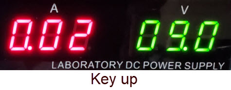
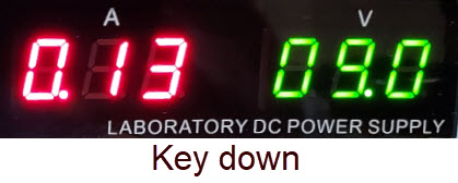 For this sub-study the ‘10-minute transmitter’ was powered from a
constant-voltage bench supply at 9 volts. The transistor used was a
2N2222A—in this simple circuit different transistors of a similar type
tend to oscillate differently. The key down power supply current
(right) was 0.13 A. Thus the circuit consumes just over one watt key
down. This observation is relevant to the feasibility of the SWR meter’s forward power reading, as
obviously RF output power cannot exceed the DC input power, and RF
voltage was not concurrently
monitored.
For this sub-study the ‘10-minute transmitter’ was powered from a
constant-voltage bench supply at 9 volts. The transistor used was a
2N2222A—in this simple circuit different transistors of a similar type
tend to oscillate differently. The key down power supply current
(right) was 0.13 A. Thus the circuit consumes just over one watt key
down. This observation is relevant to the feasibility of the SWR meter’s forward power reading, as
obviously RF output power cannot exceed the DC input power, and RF
voltage was not concurrently
monitored.

Forward
(RF) power readings varied between 193 and 211 milliwatts, while
reverse
power was below a detectable threshold. The image on the left is a
zoom view of one such forward power reading. Clearly for such readings
to be trusted
it would be necessary to calibrate the milliwatt scale independently,
by concurrently measuring
RF voltage across the load. However, as previously hinted it could be
more informative first to configure a still lower reference voltage,
and test the associated regression equation for that A-ref value’s
corresponding A/D range.

QRPps: Another
Boolean symbol was needed to distinguish the milliwatt range
in
the microcontroller code (sketch) so I added an ‘s’ to QRPp, where the
‘s’ means ‘super’ QRPp—or maybe ‘ps’ stands for ‘postscript’.
(These constants should eventually be replaced by switches.) From the
graph reproduced above it is clear that the relationship between A/D
readings and RF power is non-linear in this lowest power range. But OK, power is a function
of voltage squared, and A/D numbers correlate with RF voltage, so the
multi-point graph should
curve upwards, as it does.3
Nevertheless,
a straight-line fit is good enough for the purpose of displaying meter
readings for forward power, because the whole setup lacks reproducible
precision. RF power was computed after measuring peak-to-peak RF
voltage across the 50 ohm load, same as for the 5-watt range
calibration.
In truth I
was surprised that this test worked. During the calibration process a
radio receiver in the next room was tuned to the 10-minute
Transmitter’s frequency so that a loud and clear tone could be heard on
each key-down as the transmitter’s power-supply voltage was being
stepwise decreased. At one point the indicator LED on the transmitter
PCB went out and it took a moment to realize that the power supply had
dropped below the LED’s minimum for illumination! Even at 1.5 volts
(the lowest that the bench supply would indicate) the transmitter was
being picked up clearly on the nearby receiver.
At the outset it was not clear whether the SWR bridge from Kits and
Parts (dot com) could be used to make milliwatt power measurements
without additional modification. However, thanks to the fact that the
Nano’s analog reference could accept a suitably low comparison value,
milliwatt measurements were straightforward. The lowest RF power
detected via the Nano’s A/D converter was 16 milliwatts RMS (confirmed
through concurrent measurement of RF voltage), not bad for an
inexpensive kit and small number of accessory components!
Demo video: Low Power SWR Meter
1. The test source was
a Four State QRP Group Hilltopper-40
transceiver. One of my two
Hilltopper kit build projects (the 20-meter version) is described on this
page. Later in the
project, two other 5-watt range transceivers were also used for
demonstration or validation and the very low power scale was calibrated
using the ‘10-minute Transmitter’.
2.
RMS power was computed as peak-to-peak voltage squared
divided by 8 times
the load impedance. My consumer grade oscilloscope (Siglent 200 MHz)
has a computer interface, which can display numeric values for
measurements. It can also display automatic ‘cursor mode’ numeric
measurements on screen, and of course, it is possible to count grids
and
multiply by the volts per division setting. In the example illustrated
below, RF voltage was 11.4 peak-to-peak, so RMS power to the 50 ohm
dummy load for this (later) QRPp test was 11.42 ÷
(8 × 50) = 0.325 watts or 325 milliwatts.
The computation can be reversed if it is desired to compute the peak-to-peak
voltage
that corresponds to a given RMS power and impedance. The reverse
formula is Vp-p = √(8Z ∙ RMS power). For example, to set the Ten Minute
transmitter to output 100 mW (0.1 watts), assuming the impedance is 50
ohms, aim for an RF voltage = √(8×50×0.1) = √(40) or
approximately
6.3 volts peak-to-peak.
3. It is simple enough to
compute a quadratic for these data points. Begin by transforming the
power data (milliwatts) to square roots and solve the linear regression
through the transformed points. For the given data, this procedure
yields ŷ =
0.0256x +
3.10256 (left part of illustration below).
Next square this equation to obtain ŷ² (milliwatts) = .000655x² +
.15885x +
9.6258, where x
stands for raw A/D readings (right in
illustration). Once again, this numerical solution is only an example.
The relationship between A/D readings and RMS power depends on the
specific experimental setup, especially the bridge calibration and
analog reference value used.
Project descriptions on this page are intended for entertainment only.
The author makes no claim as to the accuracy or completeness of the
information presented. In no event will the author be liable for any
damages, lost effort, inability to carry out a similar project, or to
reproduce a claimed result, or anything else relating to a decision to
use the information on this page.


